Merge Sort: The Art of Divide and Conquer Sorting

Sorting is a fundamental task in computer science, whether it’s organizing a list of names, numbers, or even your music playlist. Merge Sort is one of the most elegant and reliable sorting algorithms, known for its consistent performance. It’s a divide and conquer algorithm, meaning it breaks a big problem into smaller, manageable pieces, solves them, and then combines the solutions. Let’s explore how it works, why it’s so

dependable, and when you’d want to use it.

What is Merge Sort?

Merge Sort is a sorting algorithm that takes a collection (like a list of numbers) and sorts it by:

Dividing the collection into smaller sublists.
Conquering by sorting those sublists.
Combining the sorted sublists back into a single, sorted list.

Think of it like sorting that pile of exam papers. You don’t tackle the whole stack at once. Instead, you split it into smaller piles, sort each pile, and then merge them back together in order. This divide-and-conquer approach makes Merge Sort efficient and predictable.

How Merge Sort Works: Divide, Conquer, Combine

Let’s break down the three steps of Merge Sort using a simple example: sorting the list [38, 27, 43, 3, 9, 82, 10].

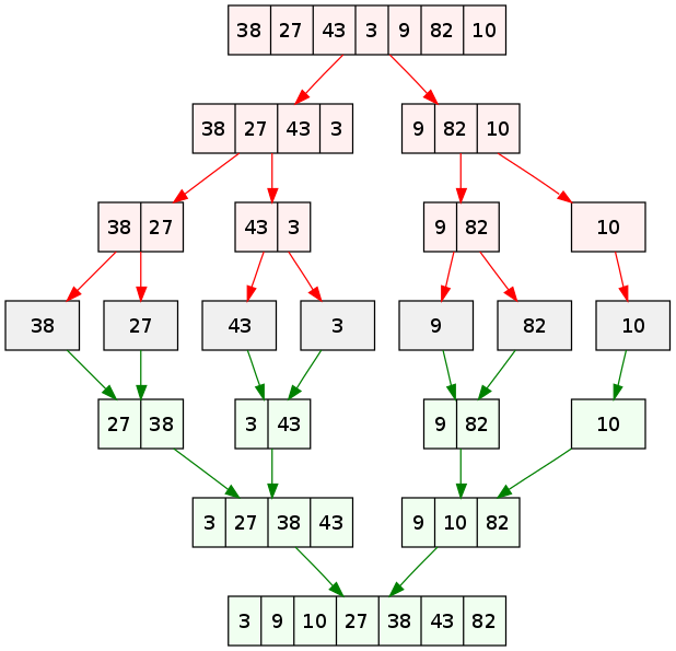
Step 1: Divide

The first step is to divide the list into smaller sublists. Merge Sort splits the list in half repeatedly until each sublist has just one element. A single-element list is already sorted (you can’t get simpler than that!).

For our list:

Start with: [38, 27, 43, 3, 9, 82, 10]
Split into: [38, 27, 43] and [3, 9, 82, 10]
Split again: [38, 27] and [43]; [3, 9] and [82, 10]
Split one more time: [38], [27], [43], [3], [9], [82], [10]

Now, each sublist has one element, and they’re all “sorted” by default.

Step 2: Conquer

The conquer step is straightforward because single-element lists are already sorted. This step sets us up for the real magic: merging.

Step 3: Combine (Merge)

The combine step is where Merge Sort shines. It takes two sorted sublists and merges them into a single sorted list. Here’s how it works:

Compare the smallest elements of each sublist.
Pick the smaller one, add it to the result, and move to the next element in that sublist.
Repeat until one sublist is empty, then append the remaining elements from the other sublist.

Let’s merge [38] and [27]:

Compare 38 and 27. 27 is smaller, so add 27 to the result: [27].
Only 38 remains, so append it: [27, 38].

Now merge [3] and [9]:

Compare 3 and 9. 3 is smaller, so add 3: [3].
Append 9: [3, 9].

Merge [82] and [10]:

Compare 82 and 10. 10 is smaller, so add 10: [10].
Append 82: [10, 82].

Now merge [27, 38] and [43]:

Compare 27 and 43. 27 is smaller, so add 27: [27].
Compare 38 and 43. 38 is smaller, so add 38: [27, 38].
Append 43: [27, 38, 43].

Merge [3, 9] and [10, 82]:

Compare 3 and 10. 3 is smaller, so add 3: [3].
Compare 9 and 10. 9 is smaller, so add 9: [3, 9].
Compare 10 (and nothing in the first list). Append 10, then 82: [3, 9, 10, 82].

Finally, merge [27, 38, 43] and [3, 9, 10, 82]:

Compare 27 and 3. 3 is smaller, so add 3: [3].
Compare 27 and 9. 9 is smaller, so add 9: [3, 9].
Compare 27 and 10. 10 is smaller, so add 10: [3, 9, 10].
Compare 27 and 82. 27 is smaller, so add 27: [3, 9, 10, 27].
Compare 38 and 82. 38 is smaller, so add 38: [3, 9, 10, 27, 38].
Compare 43 and 82. 43 is smaller, so add 43: [3, 9, 10, 27, 38, 43].
Append 82: [3, 9, 10, 27, 38, 43, 82].

The result is a fully sorted list!

Real-World Analogy

Imagine you’re organizing a huge pile of exam papers by student name. Sorting the entire stack at once is overwhelming. Instead:

Divide: Split the pile into two smaller piles. Split those piles again until you have tiny stacks of one or two papers.
Conquer: Sort each tiny stack (easy to alphabetize one or two papers).
Combine: Merge the sorted stacks by comparing the top paper of each stack, picking the one that comes first alphabetically, and building a new sorted pile.

This process is exactly how Merge Sort tackles a list, making it intuitive and systematic.

Python Code Example

Here’s a Python implementation of Merge Sort that brings the above steps to life:

Python

def merge_sort(arr):
    if len(arr) <= 1:
        return arr
    
    # Divide: Split the list in half
    mid = len(arr) // 2
    left = merge_sort(arr[:mid])  # Recursively sort left half
    right = merge_sort(arr[mid:]) # Recursively sort right half
    
    # Combine: Merge the sorted halves
    return merge(left, right)

def merge(left, right):
    result = []
    i = j = 0
    
    # Compare elements from both lists and merge in sorted order
    while i < len(left) and j < len(right):
        if left[i] <= right[j]:
            result.append(left[i])
            i += 1
        else:
            result.append(right[j])
            j += 1
    
    # Append remaining elements
    result.extend(left[i:])
    result.extend(right[j:])
    return result

# Example usage
arr = [38, 27, 43, 3, 9, 82, 10]
sorted_arr = merge_sort(arr)
print("Sorted array:", sorted_arr)

Running this code outputs: Sorted array: [3, 9, 10, 27, 38, 43, 82].

The merge_sort function handles the divide and conquer steps, while the merge function does the heavy lifting of combining sorted sublists.

Complexity Analysis

Time Complexity: O(n log n) for All Cases

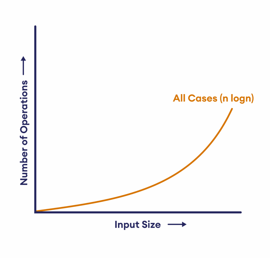
Merge Sort’s time complexity is consistently O(n log n) for best, average, and worst cases. Here’s why:

Divide: The list is split in half recursively, creating a tree of sublists. If the list has n elements, it takes log n levels to reach single-element sublists (because each split divides the size by 2).
Merge: At each level of the tree, merging all sublists requires comparing and moving n elements total. Since there are log n levels, the total work is n * log n.

Whether the list is already sorted (best case), random (average case), or reverse-sorted (worst case), the number of splits and merges remains the same. This predictability is a hallmark of Merge Sort.

Space Complexity: O(n)

Merge Sort requires extra memory to store temporary arrays during the merge process. When merging two sublists, we create a new array to hold the sorted result. In the worst case, we need space for n elements (e.g., when merging two lists of size n/2). Thus, the space complexity is O(n).

Additionally, the recursive call stack adds O(log n) space due to the depth of the recursion tree, but the dominant factor is the O(n) for the temporary arrays.

Strengths of Merge Sort

Guaranteed O(n log n): Unlike some algorithms (e.g., Quick Sort), Merge Sort’s performance doesn’t degrade with specific input patterns.
Stable Sort: It preserves the relative order of equal elements, which is crucial for sorting objects with multiple fields (e.g., sorting students by grade but keeping same-grade students in their original order).
Great for Large Datasets: Its predictable performance makes it ideal for big data, especially when data doesn’t fit in memory (external sorting).

Weaknesses of Merge Sort

Extra Space: The O(n) space requirement can be a drawback in memory-constrained environments, unlike in-place algorithms like Quick Sort.
Slightly Slower in Practice: While O(n log n), the constant factors (e.g., creating temporary arrays) make it slower than Quick Sort for average cases on smaller datasets.

Use Cases

Merge Sort is your go-to when:

You need a stable sort (e.g., sorting a list of records by one field while preserving order for others).
You’re dealing with large datasets or external sorting (e.g., sorting data on disk that doesn’t fit in memory).
You want predictable performance, regardless of input order.

It’s often used in standard library implementations (e.g., Python’s sorted() and list.sort() use a hybrid of Merge Sort and Insertion Sort called Timsort).

Conclusion

Merge Sort is like a well-organized librarian who methodically breaks down a chaotic pile of books into small, sorted stacks and merges them into a perfectly ordered shelf. Its divide-and-conquer approach ensures consistent O(n log n) performance, making it a reliable choice for sorting large or complex datasets. While it requires extra memory, its stability and predictability make it a staple in computer science. Try running the Python code above and experiment with different lists to see Merge Sort in action!

Stay tuned for the next post in our algorithm series, where we’ll explore another classic sorting technique. Happy coding!

HaMind