Searching through data is like finding a needle in a haystack, but what if the haystack is neatly organized? Interpolation Search is a brilliant algorithm that takes advantage of sorted data to make smarter guesses about where a target value might be. Unlike Binary Search, which always splits the search space in half, Interpolation Search estimates the target’s position based on the data’s distribution. In this post, we’ll break down how it works, analyze its complexity, and see why it’s a gem for certain datasets. Let’s dive in with a beginner-friendly explanation!

What is Interpolation Search?

Interpolation Search is an algorithm designed to find a target value in a sorted array (or list). It’s a step up from Binary Search, using a mathematical formula to guess where the target might be, based on the values at the array’s boundaries. Think of it as looking up a word in a dictionary: if you’re searching for “zebra,” you jump toward the end because you know “z” words are there, rather than checking the middle.

It’s not exactly a “divide and conquer” algorithm like Merge Sort or Quick Sort, but it does narrow down the search space iteratively by making informed guesses.

How Interpolation Search Works: Guess, Check, Repeat

Let’s search for the value 43 in the sorted list [3, 9, 10, 27, 38, 43, 82].

Step 1: Estimate the Position (The Interpolation Formula)

Interpolation Search assumes the data is sorted and roughly uniformly distributed (like numbers spaced evenly). It uses a formula to estimate where the target value lies:

pos = low + ((target - arr[low]) * (high - low)) // (arr[high] - arr[low])

• low and high are the indices of the current search range (initially 0 and the last index).
• arr[low] and arr[high] are the values at those indices.
• target is the value we’re searching for.

For our list [3, 9, 10, 27, 38, 43, 82]:

• low = 0 (value 3), high = 6 (value 82), target = 43.
• Plug into the formula:
  pos = 0 + ((43 - 3) * (6 - 0)) // (82 - 3) = 0 + (40 * 6) // 79 ≈ 3.
• Check index 3: arr[3] = 27.

Step 2: Compare and Narrow

Compare the target (43) with the value at the estimated position (27):

• Since 43 > 27, the target must be to the right.
• Update the search range: low = 4, high = 6 (new sublist: [38, 43, 82]).

Step 3: Repeat

Apply the formula again for the new range:

• low = 4 (value 38), high = 6 (value 82), target = 43.
• pos = 4 + ((43 - 38) * (6 - 4)) // (82 - 38) = 4 + (5 * 2) // 44 ≈ 4.
• Check index 4: arr[4] = 38.

Since 43 > 38, move right: low = 5, high = 6.

• New formula: pos = 5 + ((43 - 43) * (6 - 5)) // (82 - 43) = 5.
• Check index 5: arr[5] = 43. Found it!

If the target isn’t found, the process continues until the search range is empty (low > high).

Real-World Analogy

Think of finding a friend’s house number on a street where houses are numbered sequentially (e.g., 1, 5, 10, 15, 20, …). If you’re looking for house 18, you don’t start at the middle house. Instead, you estimate that 18 is close to 20, so you jump near the end of the street. If you overshoot or undershoot, you adjust and try again. Interpolation Search works similarly, using the values in the array to make a smarter first guess than Binary Search.

Python Code Example

Here’s a Python implementation of Interpolation Search:

def interpolation_search(arr, target):
    low = 0
    high = len(arr) - 1
    
    while low <= high and arr[low] <= target <= arr[high]:
        # Avoid division by zero
        if low == high:
            if arr[low] == target:
                return low
            return -1
        
        # Interpolation formula
        pos = low + ((target - arr[low]) * (high - low)) // (arr[high] - arr[low])
        
        # Ensure pos is within bounds
        if pos < low or pos > high:
            return -1
        
        # Check the estimated position
        if arr[pos] == target:
            return pos
        elif arr[pos] < target:
            low = pos + 1
        else:
            high = pos - 1
    
    return -1

# Example usage
arr = [3, 9, 10, 27, 38, 43, 82]
target = 43
result = interpolation_search(arr, target)
print(f"Element {target} found at index: {result}")

Running this outputs: Element 43 found at index: 5.

The code calculates the estimated position, checks it, and adjusts the search range until the target is found or determined to be absent.

Complexity Analysis

Time Complexity

Interpolation Search’s performance depends on the data’s distribution:

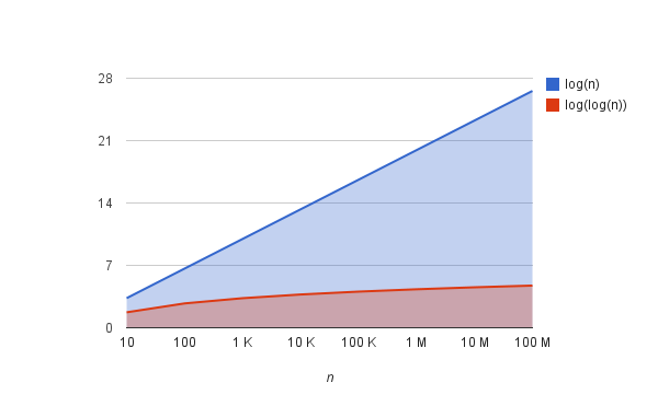
• Best Case: O(log log n)
  When the data is uniformly distributed (e.g., numbers like 1, 2, 3, …, n), the interpolation formula pinpoints the target almost perfectly, reducing the search space exponentially. This leads to O(log log n), which is incredibly fast for large, uniform datasets.
• Average Case: O(log log n)
  For roughly uniform data, Interpolation Search typically performs in O(log log n), much faster than Binary Search’s O(log n). The formula’s estimates are effective when values are spread evenly.
• Worst Case: O(n)
  If the data is poorly distributed (e.g., values like [1, 2, 3, 1000, 1000000]), the formula’s guesses can be way off, causing the algorithm to check nearly every element. This leads to O(n), similar to a linear search. For example, searching for a value far from the interpolated position can degrade performance.

The quality of the interpolation formula’s guesses is critical. Uniformly distributed data (like evenly spaced numbers) yields stellar performance, while skewed distributions hurt efficiency.

Space Complexity

• O(1) for Iterative Implementation: The iterative version (like the code above) uses a constant amount of extra space for variables (low, high, pos).
• O(log n) for Recursive Implementation: If implemented recursively, the call stack uses O(log n) space in the average case (similar to Binary Search). In the worst case, it could reach O(n) for highly skewed data.

Since the iterative version is common and simpler, Interpolation Search is typically O(1) in space.

Strengths of Interpolation Search

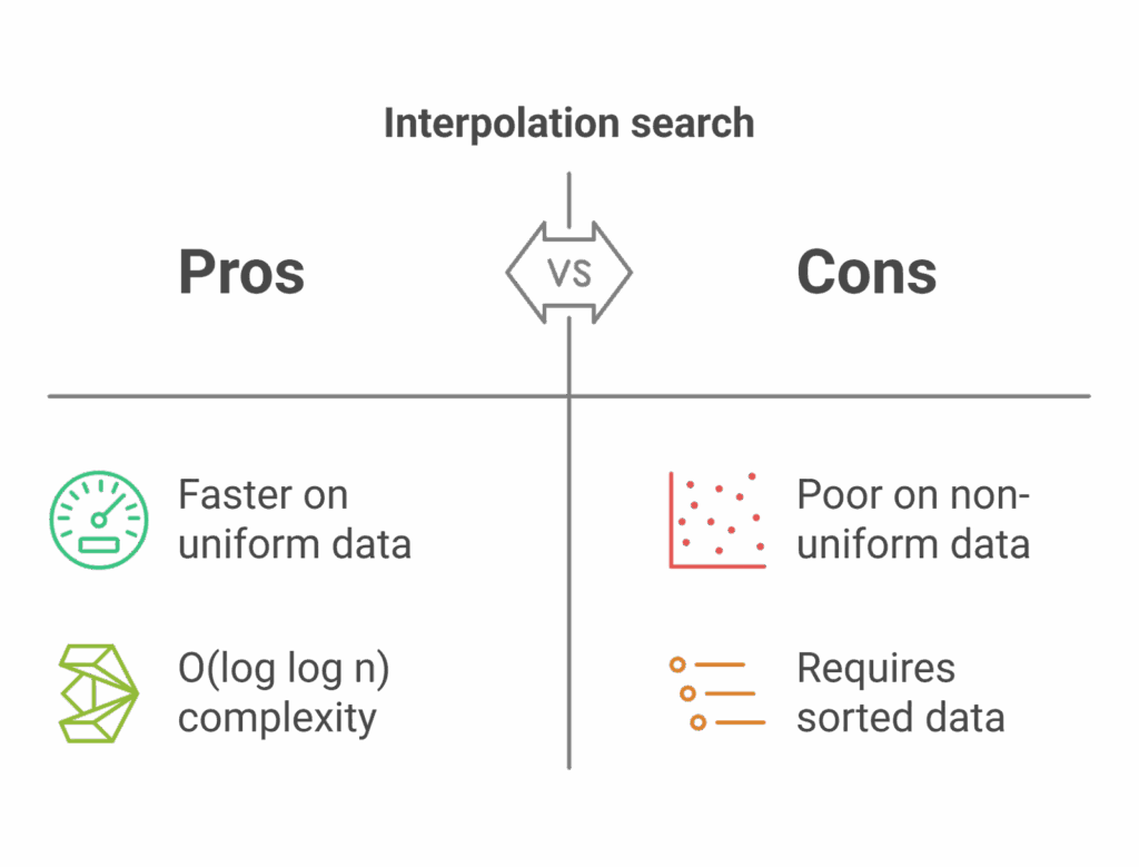
• Blazing Fast for Uniform Data: Its O(log log n) performance shines on large, uniformly distributed datasets, outpacing Binary Search.
• Simple Concept: The idea of estimating based on values is intuitive, like guessing a page in a dictionary.
• Low Space Usage: The iterative version uses constant extra space, making it memory-efficient.

Weaknesses of Interpolation Search

• Requires Sorted Data: Like Binary Search, it only works on sorted arrays.
• Sensitive to Distribution: Performance degrades to O(n) if the data isn’t uniformly distributed (e.g., exponential or irregular gaps).
• Not as General-Purpose: Binary Search is often preferred for its consistent O(log n) performance across all distributions.

Use Cases

Interpolation Search is ideal when:

• The data is sorted and uniformly distributed (e.g., evenly spaced numbers, like a list of house numbers or database keys).
• You need fast searches on large datasets where Binary Search’s O(log n) feels too slow.
• Memory is limited, as it’s space-efficient.

It’s used in scenarios like searching numerical databases or indexes with predictable patterns, but Binary Search is often favored for general-purpose use due to its reliability across distributions.

Conclusion

Interpolation Search is like a savvy librarian who guesses exactly where a book might be based on its title, jumping closer to the target with each try. Its O(log log n) performance makes it a superstar for uniformly distributed sorted data, though it stumbles with irregular distributions. Try running the Python code above with different sorted lists to see how it performs, especially with evenly spaced numbers!

Stay tuned for the next post in our algorithm series, where we’ll explore another exciting technique. Happy searching!