You’re already writing code that works, which is fantastic! But as you move forward in your careers, you’ll encounter challenges where simply working isn’t enough. You’ll need code that performs well, even when dealing with massive amounts of data. This is where a fundamental concept comes in: Algorithm Complexity.

Don’t let the fancy name scare you! Think of it as a way to predict how your code will behave when you throw a lot of data at it, without actually having to run it for hours (or days!).

What Exactly is Algorithm Complexity?

At its core, algorithm complexity is about understanding the resources an algorithm uses as the size of the input grows. When we talk about resources in this context, we primarily mean two things:

1. Time: How long does the algorithm take to run?
2. Space: How much memory does the algorithm need?

So, algorithm complexity is a measure of how “expensive” an algorithm is in terms of time and space, relative to the size of the problem it’s trying to solve.

Imagine you have a recipe (that’s your algorithm!) for making a cake.

• Making a small cupcake (n=1) takes a certain amount of time and uses a small bowl.
• Making a regular cake (n=10 servings) takes more time and a bigger bowl.
• Making a giant wedding cake (n=100 servings) takes significantly more time (maybe you need multiple ovens, more mixing, etc.) and much larger containers.

Algorithm complexity helps us predict how much more time and space are needed as the cake size (n) increases.

The Two Main Types: Time and Space

While there are other specialized types, for most practical purposes as a developer, you’ll focus on these two:

1. Time Complexity: This measures how the execution time of an algorithm increases with the input size (n). We don’t measure in seconds or milliseconds because that depends on the computer’s speed, the programming language, and even what other programs are running. Instead, we count the number of fundamental operations (like comparisons, assignments, arithmetic calculations) the algorithm performs.
2. Space Complexity: This measures how the memory used by an algorithm increases with the input size (n). This includes the space needed for variables, data structures, and function calls on the call stack.

Understanding both is important, as sometimes you can trade one for the other (e.g., using more memory to store pre-calculated results can save computation time). But often, time complexity is the first thing developers consider for performance optimization.

How Do We Talk About Complexity? Enter Big O Notation!

Okay, so we know we’re looking at how time/space grows with input size n. But how do we describe this growth? We use something called Big O notation (written as O()).

Big O notation gives us an upper bound on the growth rate. It tells us the worst-case scenario for how the algorithm’s resource usage will increase as n gets very large. We focus on the term that grows the fastest and ignore constant factors or lower-order terms because they become insignificant for large inputs.

Here are some common Big O classes you’ll encounter, from fastest (best) to slowest (worst) performance as n grows:

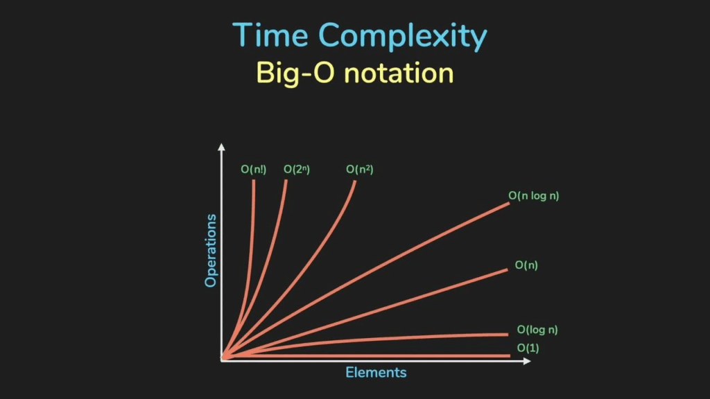
• O(1) – Constant Time: The time/space required is the same, no matter how big the input is. Super fast!
  • Analogy: Opening a specific page in a book if you know the page number. It takes the same effort regardless of how many pages are in the book.
• O(logn) – Logarithmic Time: The time/space grows very slowly as the input size increases. This usually happens when the algorithm repeatedly divides the problem size by a constant factor (like 2).
  • Analogy: Finding a word in a dictionary. You don’t check every word; you open to a page, and depending on the word, you go to the first or second half, and repeat. The number of steps increases slowly with the number of words.
• O(n) – Linear Time: The time/space grows directly proportional to the input size. If you double the input, the time/space roughly doubles.
  • Analogy: Reading every word in a book. The time it takes is directly proportional to the number of words.
• O(nlogn) – Log-Linear Time: A bit slower than linear, but still considered efficient for many tasks like sorting.
  • Analogy: Sorting a deck of cards efficiently (e.g., Merge Sort).
• O(n2) – Quadratic Time: The time/space grows with the square of the input size. Often seen in algorithms with nested loops where each loop iterates over the input. This gets slow very quickly for larger inputs.
  • Analogy: Comparing every card in a deck to every other card.
• O(2n) – Exponential Time: The time/space doubles with each additional element in the input. These algorithms are only practical for very small input sizes.
• O(n!) – Factorial Time: Grows incredibly fast. Impractical for almost any real-world input size beyond very small ones.

How Do You Use This Knowledge?

Understanding algorithm complexity helps you:

1. Compare Algorithms: If you have two different ways to solve the same problem, comparing their time and space complexity tells you which one is likely to perform better for large inputs.
2. Predict Performance: Without running your code on a massive dataset, you can get an idea of whether it will be fast enough.
3. Identify Bottlenecks: Complexity analysis can help you pinpoint parts of your code that will become slow as the input grows.
4. Write Better Code: By being mindful of complexity, you can often choose or design algorithms that are more efficient from the start.

Real-World Application: Why Does This Matter Beyond Academia?

Okay, I’m building a web app! How does O(n2) affect me? A lot!

• User Experience: A slow algorithm processing user data means your app feels sluggish. Users hate waiting.
• Scalability: If your algorithm’s time complexity is high (like O(n2) or worse), your application will struggle or become unusable as the number of users or the amount of data they generate increases.
• Cost: In cloud computing, you pay for the resources you use (CPU time, memory). Inefficient algorithms consume more resources, costing you more money!
• Battery Life: For mobile apps, inefficient algorithms can drain battery faster.

Thinking about complexity is not just an academic exercise; it’s a crucial skill for building robust, scalable, and performant software.

Putting it into Practice: Examples in Python

Let’s look at a couple of simple Python examples and analyze their time complexity.

Example 1: Accessing an element in a list

Python

my_list = [10, 20, 30, 40, 50]
element = my_list[2] # Accessing the element at index 2
print(element)

No matter how long my_list is, accessing an element by its index takes the same amount of time. This is because computers can directly jump to any memory location if they know its address (which is calculated from the starting address of the list and the index).

• Time Complexity: O(1) – Constant Time. Fantastic!

Now, let’s compare it to finding an element by its value in an unsorted list:

Python

my_list = [10, 20, 30, 40, 50]
target = 40

found = False
for item in my_list:
  if item == target:
    found = True
    break

print(found)

In the worst case, the target might be the last element, or not in the list at all. The code has to check every single element in the list.

• Time Complexity: O(n) – Linear Time. The time taken scales directly with the size of the list.

Example 2: Finding if any elements are duplicates

A simple (but not the most efficient) way to do this is to compare every element with every other element.

Python

def has_duplicates_naive(list_of_items):
  n = len(list_of_items)
  for i in range(n):
    for j in range(n): # Nested loop
      if i != j and list_of_items[i] == list_of_items[j]:
        return True
  return False

my_list = [1, 2, 3, 4, 5, 2]
print(has_duplicates_naive(my_list))

Let’s analyze the loops. The outer loop runs n times. The inner loop also runs n times for each iteration of the outer loop. So, the total number of comparisons is roughly ntimesn=n2.

• Time Complexity: O(n2) – Quadratic Time. This algorithm will become very slow very quickly as the list size grows. For a list of 1000 items, it might do around 1 million comparisons!

Could we do better? Yes! We could use a set to keep track of elements we’ve seen.

Python

def has_duplicates_efficient(list_of_items):
  seen = set()
  for item in list_of_items:
    if item in seen: # Checking for membership in a set is typically O(1) on average
      return True
    seen.add(item) # Adding to a set is typically O(1) on average
  return False

my_list = [1, 2, 3, 4, 5, 2]
print(has_duplicates_efficient(my_list))

In this improved version, we iterate through the list once (O(n)). Inside the loop, checking if an item is in a set and adding an item to a set are typically very fast operations, averaging O(1). So, the dominant factor is the single loop.

• Time Complexity: O(n) – Linear Time (on average). Much better than O(n2) for large lists!

Conclusion

Understanding algorithm complexity, particularly time and space complexity using Big O notation, is a fundamental skill for any developer who wants to write efficient and scalable code. It allows you to analyze and compare algorithms, predict their performance, and make informed decisions about how to solve problems effectively, especially as data sizes increase.

Start thinking about the loops in your code, the data structures you use, and how the number of operations might grow as your input gets larger. It’s a superpower that will make you a more valuable and effective developer.