Sorting is like tidying up your desk—everything needs to find its rightful place. Quick Sort is one of the fastest and most popular sorting algorithms, thanks to its clever “divide and conquer” strategy. It picks a special element called a pivot, organizes the rest of the list around it, and recursively sorts the resulting pieces. In this post, we’ll break down how Quick Sort works, analyze its performance, and see why it’s a favorite in many systems. Let’s dive in with a clear, beginner-friendly explanation!

What is Quick Sort?

Quick Sort is a divide and conquer algorithm that sorts a list by:

1. Choosing a pivot element from the list.
2. Partitioning the other elements into two groups: those less than the pivot and those greater than it.
3. Recursively sorting the two groups.

Think of it like lining up those kids by height. You pick one kid as the pivot, split the group based on who’s shorter or taller, and keep doing this until everyone’s in order. Quick Sort’s efficiency comes from how it cleverly divides the problem into smaller chunks.

How Quick Sort Works: Pivot, Partition, Recurse

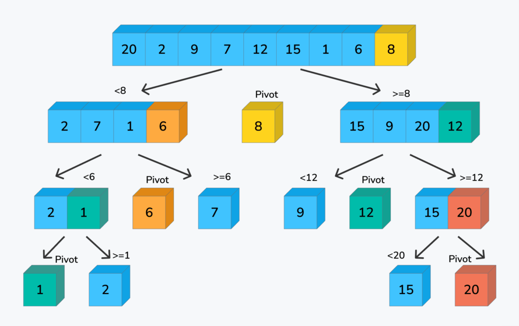
Let’s walk through Quick Sort using the list [20, 2, 9, 7, 12, 15, 1, 6, 8].

Step 1: Pivot Selection

The first step is choosing a pivot, an element that acts as a reference point. The pivot choice can affect performance, so common strategies include:

• Last element (simple but risky for sorted lists).
• First element (similar risks).
• Random element (reduces the chance of bad cases).
• Median-of-three (pick the median of the first, middle, and last elements for balance).

For our example, let’s pick the last element, 10, as the pivot. A good pivot splits the list into roughly equal parts, making the algorithm faster.

Step 2: Partitioning

The partitioning step rearranges the list so that:

• All elements less than the pivot are on its left.
• All elements greater than the pivot are on its right.
• The pivot ends up in its final sorted position.

We split the array into three parts:

• Elements less than 8 → [2, 7, 1, 6]
• The pivot → 8
• Elements greater than or equal to 8 → [15, 9, 20, 12]

Step 3: Recursive Sort

Left Sublist: [2, 7, 1, 6]

• Pivot = 6
• Partition:
  • Less than 6 → [2, 1]
  • Pivot → 6
  • Greater or equal to 6 → [7]

Now recurse on [2, 1]:

• Pivot = 1
• Partition:
  • Less than 1 → []
  • Pivot → 1
  • Greater or equal to 1 → [2]
• Combined: [1, 2]

Now combine:
→ [1, 2] + [6] + [7] = [1, 2, 6, 7]

Right Sublist: [15, 9, 20, 12]

• Pivot = 12
• Partition:
  • Less than 12 → [9]
  • Pivot → 12
  • Greater or equal to 12 → [15, 20]

Recurse on [15, 20]:

• Pivot = 20
• Partition:
  • Less than 20 → [15]
  • Pivot → 20
  • Greater → []
• Combined: [15, 20]

Now combine:
→ [9] + [12] + [15, 20] = [9, 12, 15, 20]

Final Step: Merge All

Now merge all parts:

• Left sorted: [1, 2, 6, 7]
• Pivot: 8
• Right sorted: [9, 12, 15, 20]

Real-World Analogy

Picture organizing a group of kids by height. You choose one kid (the pivot) and ask everyone shorter to stand to their left and everyone taller to their right. Once they’re split, you repeat the process for the “shorter” and “taller” groups, picking new pivots each time. Eventually, everyone’s lined up perfectly from shortest to tallest. Quick Sort does the same with numbers, splitting and sorting until the list is in order.

Python Code Example

Here’s a Python implementation of Quick Sort, using the last element as the pivot for simplicity:

def quick_sort(arr, low, high):
    if low < high:
        # Find the partition index
        pi = partition(arr, low, high)
        
        # Recursively sort the left and right sublists
        quick_sort(arr, low, pi - 1)
        quick_sort(arr, pi + 1, high)

def partition(arr, low, high):
    pivot = arr[high]  # Choose the last element as pivot
    i = low - 1  # Index of smaller element
    
    for j in range(low, high):
        # If current element is smaller than or equal to pivot
        if arr[j] <= pivot:
            i += 1  # Increment index of smaller element
            arr[i], arr[j] = arr[j], arr[i]  # Swap elements
    
    # Place pivot in its correct position
    arr[i + 1], arr[high] = arr[high], arr[i + 1]
    return i + 1  # Return pivot's index

# Example usage
arr = [20, 2, 9, 7, 12, 15, 1, 6, 8]

quick_sort(arr, 0, len(arr) - 1)
print("Sorted array:", arr)

Running this outputs: Sorted array: [1, 2, 6, 7, 8, 9, 12, 15, 20].

The quick_sort function handles the recursive calls, while partition rearranges elements around the pivot. Note that this implementation sorts in-place, modifying the original list.

Complexity Analysis

Time Complexity

Quick Sort’s performance depends heavily on the pivot choice and how it splits the list:

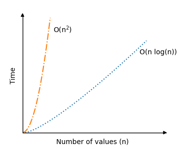
• Best Case: O(n log n)
  When the pivot splits the list into two roughly equal halves, the recursion tree has log n levels (similar to Merge Sort). Each level processes n elements during partitioning, so the total work is n * log n. This happens with good pivot choices (e.g., median or random).
• Average Case: O(n log n)
  On average, pivots create reasonably balanced partitions, leading to a recursion tree with about log n levels. The total work remains n * log n, making Quick Sort very efficient in practice.
• Worst Case: O(n²)
  If the pivot is always the smallest or largest element (e.g., in an already sorted or reverse-sorted list with a bad pivot choice like the first or last element), the list is split into one element and n-1 elements. This creates n levels, with each level doing O(n) work, resulting in n * n = n². Good pivot strategies (e.g., random or median-of-three) help avoid this.

Space Complexity

Quick Sort is mostly in-place, but the recursive call stack uses memory:

• Average Case: O(log n)
  With balanced partitions, the recursion tree has log n levels, so the call stack uses O(log n) space.
• Worst Case: O(n)
  With unbalanced partitions (e.g., sorting an already sorted list with a bad pivot), the recursion tree can have n levels, leading to O(n) space for the call stack.

Unlike Merge Sort, Quick Sort doesn’t need extra arrays for merging, making it more memory-efficient in practice.

Strengths of Quick Sort

• Super Fast in Practice: Its average-case O(n log n) performance often beats Merge Sort due to lower constant factors and in-place sorting.
• Memory Efficient: Requires minimal extra space (just the recursive call stack), unlike Merge Sort’s O(n) temporary arrays.
• Widely Used: Its speed makes it a favorite in many systems, like standard library sorts.

Weaknesses of Quick Sort

• Worst-Case O(n²): Poor pivot choices (e.g., always picking the first element for a sorted list) can lead to quadratic performance, though this is rare with good strategies.
• Not Stable: Quick Sort doesn’t preserve the relative order of equal elements, which can be an issue for certain applications.
• Trickier to Implement: Partitioning logic is more complex than simpler algorithms like Bubble Sort.

Use Cases

Quick Sort is ideal when:

• You need fast, general-purpose sorting for large datasets where stability isn’t required.
• Memory is limited, as it’s nearly in-place (unlike Merge Sort).
• You’re okay with a small risk of worst-case performance, mitigated by good pivot strategies.

It’s widely used in programming language libraries (e.g., C’s qsort) and systems where speed is critical, like sorting arrays in memory.

Conclusion

Quick Sort is like a skilled coach organizing a team by quickly splitting them into groups based on a chosen leader (the pivot) and repeating until everyone’s in place. Its average-case O(n log n) speed and low memory footprint make it a go-to for many sorting tasks, despite the rare O(n²) worst case. Try running the Python code above and experiment with different pivot strategies to see how it performs!

Stay tuned for the next post in our algorithm series, where we’ll tackle another exciting sorting technique. Happy sorting!